Engineering Study Notes

Lecture #4 Radiation from charges and currents

i. Introduction

The notes aim to derive a solution for Maxwell's equations using vector and scalar potentials. Then to express the same potentials as functions of current densities. This method alows the user to more easily obtain the electric and magnetic fields instead of directly solving Maxwell's equations. The option of presenting the E and H fields is still explored, presenting the fields in terms of the sources that create them. The second part of the notes provides insight into far-fields in terms of sources, far-field conditions and derives the radiation integrals.

ii. On notation

The notation in this note may prove to be confusing at first due to the lack of coding skills present in the author. This means that vector quantities in images containing equations will be denoted with an arrow above the letter, while the same vector quantities in the text will be denoted by the letter being in bold text. (I am sorry for the inconvenience, I will try to standardize the notation in further notes!). Also, of importance is that the differential equations given in the note are derived and shown in their phasor notation (in the complex domain). This is done for convenience and easier calculations.

1. Fields in terms of potentials

This is the first out of four parts in this lecture. Each part follows a simple process that will be given as a list of steps and then each step will be presented in detail. Part one has the following process:

Separate Maxwell's equations by electric and magnetic sources.
Derive the vector potential quantities A and F.
Solve for B_A & E_A or D_F and H_F by using the potentialls for a general medium.
Derive Helmholtz equations for A and F in a simple medium by using the Lorenz gauge.
Derive equations for E_A and H_F as functions of A and F, respectively.

Maxwell's equations in phasor notation {4-1} are the base where the reader starts the derivation. It is also important to note that a magnetic current density J_m and a magnetic charge density ρ_m are included to make the equations simmetric. These sources of magetic fields do not exist physically, but prove to be usefull when trying to calculate the fields in certain scenarios due to a law of symmerty that will be explored in future notes.

{4-1}

To derive the vector and scalar potentials Maxwell's equations are split into two sets. The first one having only electric sources (J_e & ρ_e) {4-2} and the second one having only magnetic sources (J_m & ρ_m) {4-3}.

Maxwell's equations with only electic sources

{4-2}

Maxwell's equations with only magnetic sources

{4-3}

The subscript A denotes only electic sources and the subscript F denotes only magnetic sources. In future text the note will show the methodology of deriving the vector and scalar potentials from the set of equations with electric sources {4-2}, as derivation of the potentials from equations {4-3} is analogous.

From equation {4-2} is can be seen that the divergence of the B_A field is zero. This means that the magnetic flux density can be represented as the curl of an arbitraty vector A. After that the expression for B_A can be substituted in the curl equation of the electric field intensity E_A as shown in the image below:

Derivation of the scalar electic potential and a solution for the electric field intensity

{4-4}

{4-5}

The arbitrary vector A in equation {4-5} is called the vector magnetic potential and the derived scalar ϕ_e is called the scalar electric potential. Equations {4-4} & {4-5} are valid for a general (inhomogeneous, unisotropic, non-linear) medium/materials.

If simple (homogeneous, isotropic, linear) medium/materials is assumed, the equation for H_A from {4-2} can be used to derive equaiton {4-6} for A:

Derivation of the Helmholtz equation for A potential

{4-6}

In the first row the vector identity ∇×∇×A=(∇∇⋅A-∇²A) is used. The second row utilizes the fact that the vector field A is fully defined only when its curl and divergence are known, and that it is an arbitrary non-unique field. Therefore, a condition called the Lorenz' gauge (often misspelled as Lorentz') is used allowing us to define the divergence as ∇⋅A=jωεμφ_e setting the third term in the second row to zero and thus coming to equation {4-6}. This is possible as due to the non-uniqueness of the field which means that no matter how the divergence is defined it will not have an effect on the physical field B_A.

From the third equation in set {4-2} an analogous euqation can be derived for ϕ_e as seen below:

Derivation of the Helmholtz equation for ϕ electric potential

{4-7}

Equations {4-6} and {4-7} are called inhomogeneous Helmholtz equations.

If the Lorenz' gauge defined as ∇⋅A=jωεμφ_e is substituted in {4-5} an equation for the electric intensity E_A that is a function of A only. It is important to remember that because the Lorentz' gauge is used on an equation derived in a simple medium, {4-8} is only valid for a simple medium/material.

Derivation the electric intensity E as a function of A only

{4-8}

A summary of all equations and their analogous counterparts for magnetic can be found below. The potentials derived from Maxwell's equations with magnetic sources are F the vector electric potential and φ_m the scalar magnetic potential.

Summary of the fields in terms of potentials for electric sources (1)

Summary of the fields in terms of potentials for electric sources (2)

Summary of the fields in terms of potentials for electric sources (3)

Summary of the fields in terms of potentials for magnetic sources (1)

2. Potentials in terms of currents

The second part of the lecture aims to derive equations for potentials in terms of currents/sources. The process for this part is shown in the following list:

Find a solution to the Helmholtz' PDE equations by superposition of point source solutions.
Dirac's delta function is used to derive J_e(r) as a sum (integral) of point sources J_e(r').
Solutions for A(r) and F(r) are obtained by utilizing the 3D Green's function G.
Derive solutions for B_A,H_A,E_A and D_F,H_F,E_F. Find the total fields E and H by superposition.

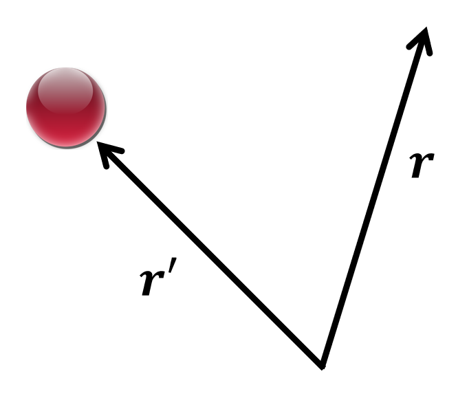
Equation {4-6} is a linear partial differential equation (PDE) and to obtain its solution a superposition of point source solutions is used. For this to happen, first, it is important to define a point source. This is done by using Dirac's delta function as shown in equation {4-9} below. The function has a value of infinity at the source and zero everywhere else. Also, to be able to derive the general case the sources will not be in the beginning of the coordinate system, meaning that there is a vector r to the observation point and vector r' to the source. The vector R = r-r' is the distance from the source to the observation point as shown in Fig. 1.

Fig. 1 Vector relations between the coordinate system, source, and observation point.

{4-9}

If the delta function δ is integrated within a volume V it will assume a value of 1 within the volume and zero everywhere else {4-10}. Equation {4-11} represents a fundamental concept in physics and applied mathematics known as the Sifting Property (or Sampling Property) of the Dirac delta function. When used, it gives the value of the function f(r) at the point r'.

Inegrating Dirac's delta function over a volume V

{4-10}

Sifting property of Dirac's delta function

{4-11}

Now it is possible to define the point source and point source densities. These are defined by using equations {4-12} and {4-13}.

{4-12}

{4-13}

To obtain a solution for the vector magnetic potential A using the Green's function method. Essentially, it shows how to calculate the potential generated by a complex distribution of current J_e by breaking it down into infinite source points.

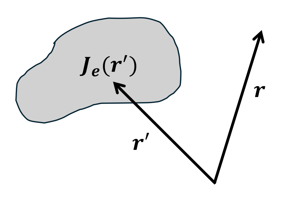
The continuous current density J_e(r) is represented as a sum(integral) of source points utilizing the Sifting property and Dirac's delta function as shown in equation {4-14} and Fig. 2.

{4-14}

Fig. 2 Vector relations between the coordinate system, current density, and observation point.

3D Green's function is the impulse response of the system. This equation defines G as the solution to the Helmholtz equation when the source is a single, unit-strength point source located at r'. If it is known how one point source behaves, it can be found how any distribution behaves. Equation {4-15} shows how Green's function is defined.

{4-15}

By substituting the current density J_e(r) eq. {4-14} and Green's function eq. {4-15} into the Helmholtz equation {4-6} asolution for the vector magnetic potential A is derived in equation {4-16}.

Vector magnetic potential in terms of current density

{4-16}

Now after a solution for A is derived, there is a need to find a solution to 3D Green's function for a poimt charge in free space. This solution is obtained by integrating equation {4-15} over a small volume around a point charge in free space. After some not-so-complicated calculations the final equation comes out in the following form {4-17}.

3D Green's function for a point source in free space

{4-17}

Green's function was the last piece needed to fully define all pieces needed to find the total Electric field E. Substituting equation {4-17} into {4-16} and then using the latter into the equations below gives solutions for B_A, E_A, and H_A. It is important to note that the second equation is valid for all space, while the third equation is only valid for source-free regions.

Before writing the solution for the total Electric field E it must be said that the process outlined in this subsection of the lecture also applies for the vector electric potential F and the quantities B_F, E_F, and H_F. The related equations are the following.

Vector electric potential in terms of current density

{4-18}

With all equations established it is time do say that the total electric and magnetic fields E and H are a superposition of the parts induced by only electric and only magnetic sources as shown in equations {4-19} and {4-20} below.

{4-19}

{4-20}

3. Fields in terms of currents